I’ve spent a fair amount of time working with Gradient Boosted Trees, and I’m comfortable enough using them to tackle most tabular problems. My understanding of neural networks, however, has remained mostly theoretical and high-level. To change this state of affairs, I decided to get my hands dirty and build something, as I am a firm believer that it is by far the best way to learn.
So here’s the challenge I set myself: on the same dataset, could I match a respectable baseline set with a GBT algorithm using a simple feed-forward neural network?
For the trees, I went with CatBoost, which everyone seem to love (I’m usually more of a LightGBM guy). PyTorch is basically the default choice for a beginner exploring neural networks, and Optuna is my go-to library for hyperparameter optimization.
And if it wasn’t clear enough already: I’m still pretty new to neural networks, and this isn’t a lesson. Think of it more as a learning log from someone exploring the fascinating world of deep learning for the first time.
Now strap in! This one’s going to be a long ride!
1. Exploring the Spaceship Titanic Dataset

For this project, I went with the Spaceship Titanic dataset from Kaggle. I never tried it before, and I liked the idea of having a public leaderboard. A little competition never hurt anyone!
Spaceship Titanic is a straightforward binary classification problem, and it’s reminiscent of the classic Titanic dataset. We will be predicting whether a passenger was "transported", a cute euphemism for "drowned". Overall, it’s a bit larger, but still very manageable: just under 8,700 rows and 13 features in the training data. The classes are well balanced (meaning as many passengers are transported as not) so there’s no need to bother with stratified splits or resampling tricks.
That said, it’s far from perfect. It’s an older synthetic dataset, and you can kind of tell. Some features that should intuitively matter, like family relationships, turn out to be completely useless, while others show surprisingly strong correlations. For instance, high spa spending is associated with being transported, while high spending in the food court predicts the opposite. And VIP status, which sounds important, barely correlates with the target variable at all. It all feels a bit random, and I’ve heard that Kaggle’s more recent synthetic datasets are much better in that regard.
For both the Gradient Boosting Trees and Neural Network parts of this post, I used the same feature-engineering setup. It’s pretty simple, partly because feature engineering isn’t the focus here, but also because the arbitrary nature of the dataset mentioned above makes it tricky to design actually helpful features. In the end, we only need solid baseline that performs well enough to place decently on the leaderboard.
Obvious First Steps
Let’s start with the low-hanging fruit. The PassengerId column follows a consistent pattern like 0001_01. The part before the underscore identifies a group of passengers traveling together, while the part after the underscore is an identifier for individuals within that group. We need to split those.
df['GroupID'] = df['PassengerId'].str.split('_').str[0].astype('Int64')
df['GroupSize'] = df.groupby('GroupID')['GroupID'].transform('count').astype('Int64')
Similarly, the Cabin column encodes the deck, the cabin number, and the side of the ship in a string like this: 'G/3/S'. That needs splitting as well:
df[['Deck', 'NumCabin', 'Side']] = df['Cabin'].str.split('/', expand=True)
df['NumCabin'] = df['NumCabin'].astype('Int64')
df['Deck'], _ = pd.factorize(df['Deck'], use_na_sentinel=True)
Ages
Let’s talk about the Age column. In the original Titanic dataset, age is a crucial predictor, so I assumed it might be just as important here. To fill in the missing values, I used a simple CatBoost regressor, which is a great fit for this kind of task thanks to its strong defaults. The idea is straightforward: train the model on passengers with a known age, using the other features as inputs, then use it to predict ages for the missing ones.
age_df = df[categorical_features + numeric_features + ['Age']].copy()
for col in categorical_features:
    age_df[col] = age_df[col].fillna("N/A").astype(str)

model = CatBoostRegressor()

model.fit(
    age_df[age_df['Age'].notna()].drop(['Age'], axis=1),
    age_df.loc[age_df['Age'].notna(), 'Age'],
    cat_features=categorical_features,
    verbose=0
)

preds = model.predict(
    age_df[age_df['Age'].isna()].drop(['Age'], axis=1)
)

df.loc[df['Age'].isna(), 'Age'] = preds
The whole thing went well, and the predicted ages are plausible. In the end, though, age turns out to be far less impactful than I expected. Time wasted? Maybe, but I prefer to think of it as a quick introduction to the CatBoost API.
A Few Constructed Features
With age values now in place, I could start adding a few simple constructed features.
df['IsChild'] = df['Age'] <= 18
df['TravellingWithAdults'] = df.groupby("Cabin")["IsChild"].transform(lambda x: (~x).sum()) - (~df["IsChild"]).astype(int)
df['TravellingWithChildren'] = df.groupby('Cabin')['IsChild'].transform('sum') - (df['IsChild']).astype(int)
IsChild does not require an explanation, but once that was was done, I wanted to use the cabin information to compute how many adults and children each passenger was traveling with. That’s what the next two features do: the number of adults (TravellingWithAdults) and children (TravellingWithChildren) sharing the same cabin. As we'll see, those features are mostly useless, but I’m keeping them anyway. I’m just too proud of that pandas code to let it go.
If It Ain’t Broke, Don’t Fix It
Let’s talk about a few feature ideas that not even pretty code could save. The first was grouping passengers by family name. It seems obvious, but it turns out that on Spaceship Titanic, family relationships don’t seem to affect transportation status at all. I also tried grouping passengers by cabin, but that information was already encoded in the first part of the PassengerId, so it doesn’t add anything new.
Then I wanted to compute a group survival rate feature. This trick works amazingly well on the original Titanic dataset, but here, groups are never split between training and test data. As a result, the feature would exist only in the training set and be entirely missing (or filled with defaults) in the test set. Useless.
Finally, I tried summing all onboard expenses (Spa, FoodCourt, etc.) into a single "total spending" feature. That turned out to be a disaster, more on that in part 5.
No NAs, No Problem
CatBoost can handle NA values natively, but PyTorch cannot, so I had to fill them manually. For this dataset, it makes sense to fill missing numeric features with 0. For example, if a passenger has a missing ShoppingMall spending amount, it’s reasonable to assume they simply didn’t spend anything. For categorical features, I filled missing values with the string UNKNOWN to create an explicit category that the models can learn from.
for feature in numeric_features:
    df[feature] = df[feature].fillna(0)
for feature in categorical_features:
    df[feature] = df[feature].fillna('UNKNOWN')
And that’s it for feature engineering. A few obvious transformations, some imputation of missing values. But the dataset should be clean enough to work well for both Neural Networks and Gradient Boosting Trees. Speaking of which, it’s time to establish a baseline!
2. Setting a Baseline Score: Gradient Boosting Trees
I won’t go into too much detail about how Gradient Boosting Trees work here; I’ll assume you already have some familiarity with the algorithm. For this project, I went with CatBoost again, because I wasn’t very familiar with it and wanted to get a better feel for it. I didn’t push too hard for maximum accuracy as the goal at this stage is simply to set a solid benchmark (and maybe land a respectable spot on the leaderboard while we’re at it!).
Preprocessing : Doing Nothing (for Trees)
Preprocessing for tree-based models couldn’t be simpler: none. Both our categorical and numeric features are completely acceptable as is. And for the love of god, please stop scaling your numeric features when using trees! MinMaxScaler and StandardScaler do literally nothing for decision trees (and yes, that’s the correct use of "literally"). Changing the distribution of the data may help however, especially if it is very skewed, but I didn't try that here.
Same goes for one-hot encoding categorical features. You won’t break anything by doing it, especially if your categories have low cardinality, but you’re just making your life harder. Modern tree implementations handle categorical features natively and far more efficiently. Instead of wasting time training on a very sparse dataset, spend it refining your feature engineering or tuning your hyperparameters. You’ll get much better returns.
Training a CatBoost Model, As Easy As It Gets
As we have seen when filling the missing values in the Age feature, training a simple model and extracting its predictions is pretty much as simple as it gets with CatBoost.
# Instantiate a CatBoost Model
model = CatBoostClassifier(
    loss_function='Logloss',
    eval_metric='Logloss',
    random_seed=SEED,
    **config                            # Hyperparameters
)

# Start Training
model.fit(
    X_train,
    y_train,
    eval_set=[(X_test, y_test)],        # Validation set for early stopping
    cat_features=categorical_features,  # Name (or indices) of categorical features
)

# Get Predictions
preds = model.predict(X_test)
I picked Logloss as the loss function (the objective to be minimized) as it much more stable for learning than simple accuracy. Once your model is instantiated with your chosen hyperparameters, all that is left is to let CatBoost do its thing.
One small thing about extracting predictions: CatBoostClassifier.predict() returns hard predictions (True / False for binary classification). If you needed predicted probabilities (floats between 0 and 1), you need to call CatBoostClassifier.predict_proba()
Finding Hyperparameters
I still wanted to score well, so I spent a bit of time tuning CatBoost’s hyperparameters with Optuna, which I am pretty new to as well. Here’s the objective function used for optimization:
def objective(trial):
    # Define the hyperparameter search space
    param = {
        'learning_rate': trial.suggest_float('learning_rate', 0.01, 0.1, log=True),
        'depth': trial.suggest_int('depth', 4, 8),                              # tree depth
        'random_strength': trial.suggest_float('random_strength', 0, 10.0),     # amount of randomness when choosing splits
        'l2_leaf_reg': trial.suggest_int('l2_leaf_reg', 0, 30),                 # L2 regularization
        'bagging_temperature': trial.suggest_float('bagging_temperature', 0.001, 10.0, log=True)  # subsampling
    }

    # Prepare cross-validation
    fold_scores = []        # will store logloss for each fold
    best_iterations = []    # will store best iteration
    kf = KFold(n_splits=5, shuffle=True, random_state=SEED)

    # Run the folds
    for fold, (train_idx, test_idx) in enumerate(kf.split(X_known, y_known)):

        # Instantiate a new CatBoost model each fold
        model = CatBoostClassifier(
            loss_function='Logloss',
            eval_metric='Logloss',
            iterations=50000,           # very high upper bound, early stopping will cut it short
            random_seed=SEED,
            **param                     # unpack Optuna's suggested hyperparameters
        )

        # Split data into train/validation for this fold
        X_train, y_train = X_known.iloc[train_idx], y_known.iloc[train_idx]
        X_valid, y_valid = X_known.iloc[test_idx], y_known.iloc[test_idx]

        # Training arguments, passed to model.fit()
        fit_param = {
            'X': X_train,
            'y': y_train,
            'eval_set': [(X_valid, y_valid)],     # validation set used for early stopping
            'cat_features': categorical_features, # names of categorical columns
            'early_stopping_rounds': 50,          # stop if no improvement for 50 rounds
            'verbose': 0
        }

        # Integrate Optuna pruning when training on the first fold only
        if fold == 0:
            pruning_callback = optuna.integration.CatBoostPruningCallback(trial, 'Logloss')
            model.fit(callbacks=[pruning_callback], **fit_param)
            pruning_callback.check_pruned()
        else:
            # For other folds, we just train normally
            model.fit(**fit_param)

        # Evaluate and store results of the folds
        preds = model.predict_proba(X_valid)
        fold_scores.append(log_loss(y_valid.to_list(), preds))
        best_iterations.append(model.get_best_iteration())

    # Report averaged metrics of all folds to Optuna
    # Store the average best iteration (useful later for retraining the final model)
    trial.set_user_attr('iterations', sum(best_iterations) / len(best_iterations))
    # Return the mean validation LogLoss across folds (the metric Optuna will minimize)
    return sum(fold_scores) / len(fold_scores)
It might look heavy, but at a high level it’s actually straightforward: for every set of hyperparameters Optuna suggests, we perform a 5-fold cross-validation. Each fold gets a fresh CatBoost model, which is trained, evaluated, and scored using Logloss. We then return the mean Logloss across folds as the objective value.
To speed things up, the function uses Optuna’s pruning system. During the first fold, it reports the model’s progress at each boosting iteration. If the performance doesn’t look promising, Optuna will order the trial to stop early, saving time by skipping both the subsequent iterations and the remaining folds. That’s why, in the optimization timeline, you’ll see several gaps: those correspond to the pruned trials that Optuna decided weren’t worth pursuing further. Running pruning on a single fold is a bit risky (you can always get an unlucky split), but I took the bet that if the first fold performs poorly, the others won’t be great either.
Another nice quality-of-life feature I used is Optuna’s ability to store custom attributes for each trial. Here, I recorded the mean of the best iteration counts across folds. Saving it here lets me train the final model with the optimal number of boosting rounds without having to rerun a (cross-) validation just to obtain it.
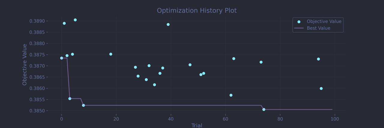
After a hundred trials, Optuna quickly converged to a solid configuration:
Best trial:
Logloss: 0.3850545609157324
Params:
learning_rate: 0.07849818024752603
depth: 6
random_strength: 0.5956085799719233
l2_leaf_reg: 14
bagging_temperature: 6.286836748473349
iterations: 459
Optuna seems to prefer giving the model quite a high number of somewhat shallow trees along with some pretty strong regularization, Speaking of which, it clearly favor l2_leaf_reg and bagging_temperature over random_strength. And the final log loss of 0.385 is very promising.
Results: A Solid Baseline To Compare With
Testing our tuned CatBoost model on a holdout test set yields the following metrics:
print(f'Accuracy: {accuracy_score(y_test, preds)}')
print(classification_report(y_test, preds))
Accuracy: 0.8148361127084531
              precision    recall  f1-score   support

         0.0       0.81      0.81      0.81       843
         1.0       0.82      0.82      0.82       896

    accuracy                           0.81      1739
   macro avg       0.81      0.81      0.81      1739
weighted avg       0.81      0.81      0.81      1739
This 0.81 accuracy is quite respectable, and as expected for this balanced dataset, there are no class imbalance issues. And on this positive note, let's leave the comforting shade of trees and step into the sunlight: it’s time to build some neural networks.
3. A Gentle Introduction to Neural Networks Architecture
For this gentle introduction, we'll start with the simplest kind there is: a fully connected Feed Forward Network, also known as a Multi-Layer Perceptron (MLP). No memory (like in RNNs), no convolution layers (like in CNNs), no attention (like in Transformers). Just layers of neurons passing numbers forward.
As mentioned in the introduction, I’ll be using PyTorch. It’s easy to install, simple to use, and widely adopted in the field. That last point shouldn’t be underestimated: when given the choice, I almost always go for the popular library, because popularity usually means better documentation, more tutorials, and plenty of helpful answers on StackOverflow.
That said, we still have a solid benchmark to hit (and plenty to learn!), so we can’t keep things too simple. Along the way, we’ll explore a few slightly more advanced topics: choice optimizers and loss functions, training in batches, dropout modules and batch normalization, network architecture tuning, and we'll even touch on embeddings for categorical features.
Anatomy of a Neural Network
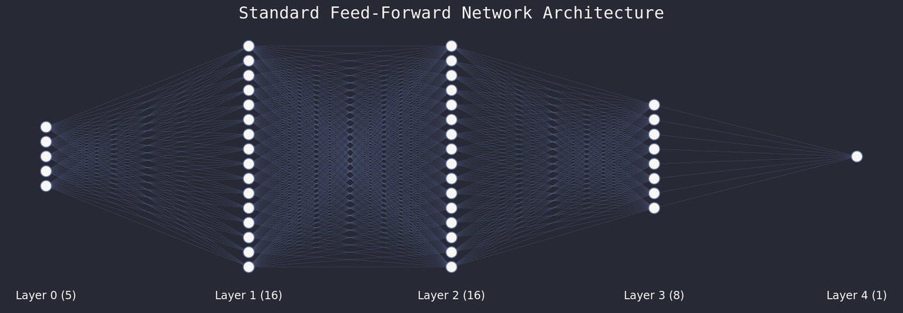
Before diving into code, let’s make sure we speak the same language. The picture above shows the classic diagram of a feed-forward network, you must have seen something similar to it already. You might even feel like you have a good understanding of what it shows, but there are some gotchas. So let's go over it anyways.
- Neurons and Activations: The nodes in the diagram are neurons. Conceptually, each neuron is like a memory cell that stores a single value: its activation.
- Layers: Neurons are grouped into layers. The input layer receives the data, with each neuron corresponding to a numeric feature (we’ll handle categories later). The output layer only contains a single neuron in our binary classification case and produces the final activation: the probability of the target being "True" (or its logit, but we’ll get to that). Every layer in between is called a hidden layer. Layers have a width (the number of neurons per layer), while the network has a depth (the number of hidden layers).
- Weights: The edges represent different concepts depending on what the network is doing. During training, the edges are the weights. Each activation in layer $L_i$ is multiplied by its corresponding weight to influence the activations in layer $L_{i+1}$. These weights are parameters updated at every learning step. In fact, the update of those weights (or more precisely, those parameters) is what learning is!
- Signals: During inference (i.e. prediction), the edges represent signals. Signals are the values that actually flow through the network: the product of the activations of the previous layer and the weights (plus biases and potentially other ingredients, which we’ll cover later).
Diagrams like this one are great for building intuition, but remember, they’re abstractions. Despite giving the algorithm its name, there are ironically no neuron living inside your GPU. Under the hood, activations are stored in arrays, and the weights between each layers are stored in a huge matrix of floats. In fact, at its core, a trained model is pretty much nothing more than a sequence of matrices transforming your inputs step by step until you get an output.
With this background, we’re ready to start building our network architecture. We’ll make it parametric, so that later we can let Optuna choose the optimal width and depth.
class SpaceTitanicNet(nn.Module):
    def __init__(self, n_input_features, width, depth, dropout_rate):
        super().__init__()

        # Layers
        self.layer_stack = nn.Sequential()

        if depth == 0:
            self.layer_stack.append(nn.Linear(n_input_features, 1))

        else:
            # depth >= 1: Input -> Hidden layers -> Output
            self.layer_stack.append(nn.Linear(n_input_features, width))
            last_hidden_size = width

            if depth >= 2 :
                # Full width hidden layers
                for i in range(depth - 2):
                    self.layer_stack.append(nn.Linear(width, width))

                # Final hidden layer at half width (if depth >= 1)
                self.layer_stack.append(nn.Linear(width, width // 2))
                last_hidden_size = width // 2

            # Output layer
            self.layer_stack.append(nn.Linear(last_hidden_size, 1))
One important thing to understand: PyTorch's nn.Linear is not a layer of neurons, but but a weight matrix (the edges between the layers on the diagram above). So at depth=0 (no hidden layer), we have a single weight matrix nn.Linear(n_input_features, 1), connecting the input neurons to the output neurons directly. At depth=1, we have two matrices, one connecting the input layer to a single hidden layer nn.Linear(n_input_features, width), and one connecting that hidden layer to the output layer nn.Linear(width, 1). And as depth increases, additional hidden layers are added.
Notice also how we taper the network as we approach the output layer. When the network has at least two hidden layers, the final hidden layer is smaller (width // 2). This is a common pattern: it progressively reduces dimensionality before the final output (which has dimension 1 in a binary classification problem).
Activation Functions: Teaching the Network to Bend
Let's think about the signal that is propagated through our layers at the neuron level. As we have seen above, for any single neuron of layer $L_{i+1}$, its activation $z$ is going to be the weighted sum of all activations in layer $L_i$. But one thing I glossed over is that each neuron also gets a bias. The bias is, just like the weights, a parameter that gets added to the activation. And just like any parameters, it gets learned by the network. As a math equation, the whole thing looks like this:
$$z = w_1a_1 + w_2a_2 + ... + w_na_n + b$$
where $a_1, a_2, ..., a_n$ are the activations of the neurons on layer $L_i$, $w_1, w_2, ..., w_n$ are the weights between layers $L_i$ and $L_{i+1}$ and $b$ is the bias. That can be written more simply in a matrix form like this:
$$Z = WA_L + b$$
It now looks suspiciously similar to a very simple affine function $f(x) = ax + b$! By default, PyTorch’s nn.Linear actually performs this affine transformation (though you could disable the bias parameter to get a purely linear transformation).
Let's now try to think about what happens in the whole network instead of a single layer. We are going to work with a network with a single hidden layer, and $X$ is going to be the input vector (the list of input values, fed in the network as the activations of our input layer). We have 2 transformation happening: $Z_1$ from the input layer to the hidden layer, and $Z_2$ from the hidden layer to the output layer: $$Z_1 = W_1X + b_1$$ $$Z_2 = W_2Z_1 + b_2$$ We can substitute $Z_1$ into $Z_2$ to get a single transformation: $$Z_2 = W_2(W_1X + b_1) + b_2$$ $$Z_2 = (W_2W_1X)x + (W_2b_1 + b2)$$ And that is still an affine transformation!
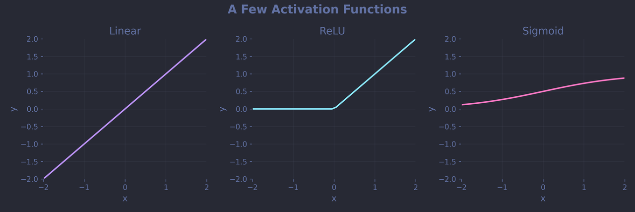
I hope I haven’t lost anyone in the maths (which, I promise, are almost over). The key takeaway is this: no matter how many hidden layers you stack, a network made only of linear layers can still model only linear relationships. For instance, it could learn something simple like "the likelihood of transportation increases with the passenger’s shopping mall spending", but it couldn’t capture more complex pattern, such as "high spending increases transportation likelihood, but low and zero spending have roughly the same effect".
To model those non-linear relationships, we need to add a bit of non-linearity, through the use of activation functions. One of the simplest and most popular is the Rectified Linear Unit (ReLU): $\phi(z) = max(0,z)$. It zeroes out any negative value and passes positive ones unchanged.
Conceptually, you can think of it as an other transformation that happens in the edges between neuron layers in the network diagram, but at the hardware level, it's much more efficient to compute the weighted sum and the activation function independently. So when it finally comes time to add non-linear activation to our linear layers (which you'd typically do for each of them except the last one), the code will look like this (for a network of depth=1):
# Layers
self.layer_stack = nn.Sequential()
self.layer_stack.append(nn.Linear(n_input_features, width))
self.layer_stack.append(nn.ReLU()) # The ReLU non-linear activation function
self.layer_stack.append(nn.Linear(width, 1))
# No ReLU after the output layer
Refining the Model: Dropout and Batch Normalization
For those who don't know about it, DART, in the context of Gradient Boosting Trees, is a technique in which entire trees are dropped randomly during training so that no single tree too important. Doing this helps regularize the ensemble, forcing the remaining trees to compensate and improving generalization. Well, a dropout layer does a similar same thing for neural networks: instead of dropping trees, we randomly ignore some neurons' outputs during training. The results are the same, preventing the network from becoming too dependent on specific neurons and thus helping it learn more robust and generalizable patterns.
In PyTorch, dropout is one of the simplest regularization tools to use:
self.layer_stack = nn.Sequential()
self.layer_stack.append(nn.Linear(n_input_features, width))
self.layer_stack.append(nn.ReLU())
self.layer_stack.append(nn.Dropout(dropout_rate)) # Our new dropout layer
You typically insert it after each hidden layer, but not after the input or output layers. dropout_rate is the probability of each neuron in the layer to be completely ignored. We'll let Optuna set it appropriately.
And now, let's talk about batch normalization. It's a technique introduced by Google engineers in 2015 and described in detail in their landmark paper. To understand what it does, you first need a rough idea of the problem it solves. Without it, the distribution of activations inside a network during training tends to shift as earlier layers learn. This makes training unstable and forces later layers to keep adapting to constantly changing inputs. If the network is not able to adapt fast enough, the activations of latter layers either explode of disappear. This phenomenon is known as internal covariate shift.
Batch normalization fixes this by acting like a learnable version of StandardScaler applied to a layer’s activations. It keeps activations within a stable range by standardizing them, while allowing the network to fine-tune that range through two learned parameters that scale and shift the normalized values.
The concept can feel a bit abstract, especially since we haven’t talked about batches yet, but the important thing for now is that, thanks to PyTorch, adding batch normalization to our network is dead simple:
self.layer_stack = nn.Sequential()
self.layer_stack.append(nn.Linear(n_input_features, width))
self.layer_stack.append(nn.BatchNorm1d(width)) # Batch Normalization Layer
self.layer_stack.append(nn.ReLU())
self.layer_stack.append(nn.Dropout(dropout_rate))
Bringing the Pieces Together: Our First Model
We now have all the pieces we need to build our network. We'll keep the architecture we had, and just add activation function, dropout and batch normalization modules where it makes sense.
class SpaceTitanicNet(nn.Module):
    def __init__(self, n_input_features, width, depth, dropout_rate):
        super().__init__()

        # Layers
        self.layer_stack = nn.Sequential()

        if depth == 0:
            self.layer_stack.append(nn.Linear(n_input_features, 1))

        else:
            # depth >= 1: Input -> Hidden layers -> Output
            self.layer_stack.append(nn.Linear(n_input_features, width))
            self.layer_stack.append(nn.BatchNorm1d(width))
            self.layer_stack.append(nn.ReLU())
            self.layer_stack.append(nn.Dropout(dropout_rate))
            last_hidden_size = width

            # Full width hidden layers
            if depth >= 2 :
                last_hidden_size = width // 2

                for i in range(depth - 2):
                    self.layer_stack.append(nn.Linear(width, width))
                    self.layer_stack.append(nn.BatchNorm1d(width))
                    self.layer_stack.append(nn.ReLU())
                    self.layer_stack.append(nn.Dropout(dropout_rate))

                # Final hidden layer at half width (if depth >= 1)
                self.layer_stack.append(nn.Linear(width, width // 2))
                self.layer_stack.append(nn.BatchNorm1d(width // 2))
                self.layer_stack.append(nn.ReLU())
                self.layer_stack.append(nn.Dropout(dropout_rate))

            # Output layer
            self.layer_stack.append(nn.Linear(last_hidden_size, 1))
And with our model defined, we are getting close to being able to train it!
4. Teaching the Network to Learn
At a high level, training neural networks happens in four steps.
- Forward pass: The network receives a set of inputs and produces predictions, just like during inference.
- Loss computation: This part should be very familiar. We measure how far those predictions are from the true values using a loss function.
- Backpropagation: I am not going to even attempt to explain the algorithm in here, but the idea is that this is how the network figures out how much each weight contributed to the error and computes how each should change to reduce it. These directions of change are called gradients.
- Optimizer step: The optimizer uses those gradients to slightly adjust the weights, strategically moving them toward values that minimize the loss.
This cycle repeats thousands of times, with each cycle nudging the network’s parameters a little closer to the configuration the produces the smallest error.
Luckily, PyTorch takes care of most of the heavy lifting. Our job is simply to define what happens in the forward pass, choose an appropriate loss function and optimizer, and write the training loop to bring it all together.
The Forward Pass
Asking the model to make a prediction (whether during training or inference) is as simple as calling model(X). Under the hood, PyTorch will look for a forward() method in your model class and call it with the input data. The role of forward() is to define the exact sequence of transformations that should be applied to the input.
In our case, all layers are already neatly arranged inside an nn.Sequential object. You can think of it as a pipeline of modules (linear layers, activations, normalizations, and so on), where the output of one becomes the input of the next. Assuming the input data is all numeric, this structure allows us to write a pretty trivial forward() method.
class SpaceTitanicNet(nn.Module):
    def __init__(self, n_input_features, width, depth, dropout_rate):
        # Layers
        # Same as above
        ...

    def forward(self, x):
        x = self.layer_stack(x)  # Pass through all layers and modules sequentially
        return x.squeeze(1)      # Remove trailing dimension: shape [batch_size]
Loss Function and Optimizer
Just like with our CatBoost model, we’ll measure error using a form of log-loss. In PyTorch, the basic option for binary classification is Binary Cross-Entropy Loss (nn.BCELoss). It is however recommended to use the more "numerically stable" alternative Binary Cross-Entropy with Logits (nn.BCEWithLogitsLoss).
What’s the difference? Earlier, I mentioned that the activation of our output neuron isn’t a probability but a raw score called a logit. To convert that logit into a probability, we would normally apply a sigmoid activation function. We could add a sigmoid layer at the end of the model layer stack, but during training, it’s actually better to skip it and let the loss function work with logits directly. So, the plan is to keep the model’s output as logits during training for nn.BCEWithLogitsLoss, and only apply the sigmoid at inference time when we actually need probabilities.
We also need an optimizer. PyTorch offers many options (full list here), but we'll keep things simple and stick with a modern and popular choice for a vast range of problems, the Adam optimizer.
Here’s a small helper function that bundles everything together:
def create_model(width, depth, lr, dropout_rate):
    model = SpaceTitanicNet(
        n_input_features=n_input_features,
        width=width,
        depth=depth,
        dropout_rate=dropout_rate
    )

    loss_fn = nn.BCEWithLogitsLoss()
    optimizer = torch.optim.Adam(model.parameters(), lr=lr)

    return model, loss_fn, optimizer
The Simplest Training Loop Possible
All the building blocks are finally in place, it is time to write our first, very simple training loop. Remember the four steps of training? Forward -> Loss Computation -> Backpropagation -> Optimizer step. Well here they are, in code:
# Instantiate our model, loss function and optimizer
model, loss_fn, optimizer = create_model(width=32, depth=2, lr=0.1, dropout_rate=0.1)

# Set our network in training mode
model.train()

# Training for 10 epochs (10 complete passes through the training set)
for epoch in range(10):
    # Forward pass: get predictions for X_train
    preds = model(X_train)

    # Loss Computation between predictions and true labels
    loss = loss_fn(preds, y_train)

    # Clear old gradients
    optimizer.zero_grad()

    # Backpropagation: compute gradients
    loss.backward()

    # Optimizer step: Update weights
    optimizer.step()
Each full pass through the training data is called an epoch. After each epoch, the model (hopefully) becomes a little more accurate.
Once training is complete and we’re ready for inference, we need to switch the network to evaluation mode. This tells PyTorch to disable certain training-specific behaviors (such as dropout and batch normalization updates) that should not run during inference.
# Set network in evaluation mode
model.eval()

# Disable gradient computation for performance
with torch.no_grad():
    # Apply sigmoid to turn logits into probabilities
    preds = torch.sigmoid(model(X_test))

# Optional: convert probabilities to binary predictions
preds = torch.round(preds)
And there we have it: a working training loop! We’re almost ready to look at some results, but not quite yet! The attentive reader will have noticed that we’ve completely skipped the data preparation step.
5. Preparing Data for the Network
Preparing data for neural networks is usually a bit more hands-on than for tree-based models. They’re fussier about both data quality and structure, and demand a bit more care before training can begin.
Data Preprocessing
Unlike most modern tree implementations, PyTorch models don’t handle categorical features natively. At this stage, we’ll simply convert each category into an integer ID. We could feed those directly into the network, but that’s really not ideal, and we’ll work on a better solution in the next chapter.
cat_maps = {}
for feature in categorical_features:
    dnn_df[feature], uniques = pd.factorize(dnn_df[feature])
    cat_maps[feature] = uniques
Also unlike trees, neural networks are very sensitive to the scale of numeric features. A good first step is to standardize them. Most of the time, using a single scaler for all the numeric features is preferable, as it preserves the relative distributions between them.
scaler = StandardScaler()
dnn_df[numeric_features] = scaler.fit_transform(dnn_df[numeric_features])
Since I concatenate the training and test data before feature engineering (to avoid doing everything twice), I now need to split them back apart.
known_mask = dnn_df['Transported'].notna()
X_known = dnn_df.loc[known_mask, categorical_features + numeric_features]
y_known = dnn_df.loc[known_mask, 'Transported'].astype(float)
X_unknown = dnn_df.loc[~known_mask, categorical_features + numeric_features]
Finally, we need to transform these dataframes into tensors. We haven’t formally introduced tensors yet, but for the purpose of this article, you can think of them as NumPy arrays optimized for neural network operations.
X_known = torch.tensor(X_known.values, dtype=torch.float32)
y_known = torch.tensor(y_known.values, dtype=torch.float32)
X_unknown_tensor = torch.tensor(X_unknown.values, dtype=torch.float32)
Dataset and Batch Training
In our previous training loop, we iterated over epochs. As mentioned at the time, those are complete passes through the entire training dataset. That works, but splitting the data into batches comes with several advantages.
The main one is speed: parameter updates happen after each batch instead of after each epoch, which helps the model converge faster. It also reduces memory usage, an important factor when working with large datasets on GPUs. Batch training also acts as a form of regularization (much like the bagging_fraction parameter in tree models), since each update is based on a subset of the data. And, of course, it’s what allows our Batch Normalization layers to function correctly. Remember those?
While we could manually slice our tensors into batches, PyTorch offers a much cleaner approach through the Dataset and DataLoader classes. First, let's create a very simple Dataset:
class SpaceTitanicDataset(Dataset):
    def __init__(self, X, y):
        self.X = X
        self.y = y

    def __len__(self):
        return len(self.y)

    def __getitem__(self, idx):
        return self.X[idx], self.y[idx]

dataset_known = SpaceTitanicDataset(
    torch.tensor(X_known.values, dtype=torch.float32),
    torch.tensor(y_known.values, dtype=torch.float32)
)
Data without known targets (the Kaggle test set in this case) can stay as a plain tensor for now, though it is also possible to batch inference later if needed. Now, let’s update our training loop. We'll instantiate a a DataLoader, which handles the batching and the shuffling of our Dataset automagically. While we are at it, let's also encapsulate the training logic in a convenient helper function:
# Split dataset into train/test
train_size = int(0.8 * len(dataset_known))
test_size = len(dataset_known) - train_size

train_dataset, test_dataset = random_split(
    dataset_known, [train_size, test_size], generator=torch.Generator().manual_seed(SEED)
)

def train_model(dataset, epochs, batch_size, width, depth, lr, dropout_rate):
    dataloader = DataLoader(dataset, batch_size=batch_size, shuffle=True)
    model, loss_fn, optimizer = create_model(width, depth, lr, dropout_rate)
    model.train()
    for epoch in trange(epochs, desc="Epoch"): # For each epoch (full pass through the data)
        for X_batch, y_batch in dataloader:    # For each batch (pass through a sample of the data)
            preds = model(X_batch)
            loss = loss_fn(preds, y_batch)
            optimizer.zero_grad()
            loss.backward()
            optimizer.step()
    return model

model = train_model(train_dataset, **config)

X_test, y_test = test_dataset[:]
model.eval()
with torch.no_grad():
    preds = model(X_test)
preds = torch.round(torch.sigmoid(preds))
6. Embeddings: The Right Way to Deal With (Most) Categories
In the previous chapter, we encoded categorical features as increasing integers. That works for a quick test, but it introduces a problem: those numbers imply an ordered relationship that probably doesn’t exist. If you label Earth = 0, Mars = 1, and Europa = 2, the model might infer that "Earth < Mars < Europa" carries some meaning, even though there’s no actual hierarchy between planets.
A common workaround is one-hot encoding, which creates a boolean column for each category. Mathematically, each category becomes a unit vector in a space whose dimensionality equals the number of categories. For example, one-hot encoding the HomePlanet feature would produce four orthogonal vectors (one per planet) in a four-dimensional space. It works, but it’s incredibly wasteful for high-cardinality features. Imagine training a language model this way, where every word (or more accurately token) would need its own dimension!
Instead of assigning each category its own axis in a massively high dimensional space, we could map categories into a lower-dimensional vector space. Imagine every passenger from Mars and Earth was transported, but every passenger from Europa was not. We could represent the passengers' home planet in a one-dimensional space by assigning Mars and Earth the same unit vector and Europa the opposite one. That would be preserving all of the relevant information with the least amount of data.
So far, all of this should sound familiar if you’ve worked with dimensionality reduction techniques like PCA. What's new here is that we can let the network learn the optimal vectors to represent each category in the vector space. In that case the vectors are called embeddings and the space itself is the embedding space. Embeddings are parameters of the network, and just like any other parameters (such as weights), they get updated through the backpropagation algorithm and the optimizer step.
If I just lost you somewhere in high-dimensional space, don’t worry, here’s what you need to know: we’re replacing a whole bunch of one-hot columns for each category with just a few numeric features learned by the network that (hopefully) capture the same amount relevant information, and make life easier for the network.
Still a bit abstract? Let’s visualize it!
So what are we seeing here? Luckily, our categorical features only contain 3 to 4 categories each, so we can squeeze them into 2-D embedding spaces and visualize them easily. For each feature, I created that two-dimensional embedding and plotted the vectors corresponding to each category after training. The scale of each plot isn’t consistent across embedding spaces, but that’s fine, since magnitude of embeddings can’t meaningfully be compared across embedding spaces anyway.
When you hover over the picture, you should see an animation: the vectors are drifting as the network learns useful coordinates for itself, batch after batch. They start at random, and although the motion is a bit noisy, it’s clear that the network has chosen to keep the categories of both CryoSleep and Side very far apart. It's also interesting to notice that it had done the same for all the known categories of HomePlanet, but has chosen to group slightly closer the 'UNKNOWN' category to 'Earth', maybe suggesting closer outcomes than with the other two.
Now, to be fair, with such small categorical variables, one-hot encoding would have worked perfectly well (and might even have performed slightly better). Also, note that creating embedding spaces for strictly boolean features is completely pointless: you’d just be converting a one-dimensional category into a one-dimensional embedding.
That said, I hope you’re now convinced of the power of embeddings (at least conceptually) and ready to make them happen in code! We’ll need to tweak our network definition to make use of them.
class SpaceTitanicNet(nn.Module):
    def __init__(self, cat_maps, numeric_features_count, width, depth, dropout_rate):
        super().__init__()

        self.categorical_features = list(cat_maps.keys())
        self.n_cats = len(self.categorical_features)

        # Embeddings
        embeddings = []
        for feature in self.categorical_features: # One embedding space for each categorical features
            num_categories = len(cat_maps[feature])
            embedding_size = min(50, (num_categories + 1) // 2) # Manually chose the dimensionality of the embedding
            embeddings.append(nn.Embedding(num_categories, embedding_size))

        self.embeddings = nn.ModuleList(embeddings)
        # Number of input neurons corresponding to every embedding
        total_embeddings_size = sum([e.embedding_dim for e in self.embeddings])

        n_input_features = total_embeddings_size + numeric_features_count
        # Layers are unchanged
        ...
We added a nn.ModuleList which is very similar to a nn.Sequential to store our embedding spaces (nn.Embedding). The dimensionality of each embedding space follows a classic rule of thumb $dimensionality = min(50, (cardinality + 1) // 2)$. Once those are created, we need to update the size of our input layer, since each categorical feature will contribute one input neuron per corresponding embedding space dimension.
Let’s now adjust our forward() method:
def forward(self, X):
    # Split categorical and numeric features
    X_cats = X[:, :self.n_cats].long()
    X_nums = X[:, self.n_cats:]

    # Embeddings
    embeddings_vectors = []
    for feature, embedding in enumerate(self.embeddings):
        cat_codes = X_cats[:, feature]
        embeddings_vectors.append(embedding(cat_codes))

    embeddings_vectors_concat = torch.cat(embeddings_vectors, dim=1)
    x = torch.cat([embeddings_vectors_concat, X_nums], dim=1)

    x = self.layer_stack(x)
    return x.squeeze(1)
Here, we split our input between categorical and numeric features. For each categorical feature, we retrieve the corresponding embedding (a vector) based on its category index. Then, we concatenate all the embedding vectors together, along with the numeric features, to form a single tensor ready to be fed into the input layer.
I know that was quite a lot, but we are getting there. Embeddings are a really powerful technique, which you should really get familiar with if you want to push your models to the next level. And a nice bonus is that embeddings aren’t just for neural networks. It’s actually quite common to use a neural network to pre-train embeddings for categorical features, then feed those learned vectors into a tree-based model. You can see an example of this approach in the YDF (formerly TF-DF) documentation.
7. Hyperparamter Optimization
Believe it or not, we’re done tinkering with the model. There’s always room for improvement, but at this point, the architecture should be solid enough to be competitive with our benchmark. Before we start actually training it, though, let’s tune some hyperparameters.
The process is conceptually identical to what we did with CatBoost: the model has several knobs to turn, and we want to find the combination that minimizes our chosen metric.
Here’s our Optuna objective function, adapted for the neural network:
def objective(trial):
    config = {
        'batch_size': trial.suggest_categorical('batch_size', [2 ** i for i in range(6, 10)]),
        'width': trial.suggest_int('width', 8, 512, step=2),
        'depth': trial.suggest_int('depth', 1, 5),
        'lr': trial.suggest_float('lr', 1e-4, 1e-1, log=True),
        'dropout_rate': trial.suggest_float('dropout_rate', 0.1, 0.7)
    }

    fold_scores = []
    best_epochs = []
    kf = KFold(n_splits=5, shuffle=True, random_state=SEED)

    # For each fold
    for fold, (train_idx, valid_idx) in enumerate(kf.split(X_known)):
        train_dataset = Subset(dataset_known, train_idx)
        valid_dataset = Subset(dataset_known, valid_idx)
        train_dataloader = DataLoader(train_dataset, batch_size=config['batch_size'], shuffle=True)
        valid_dataloader = DataLoader(valid_dataset, batch_size=config['batch_size'], shuffle=False)

        model, loss_fn, optimizer = create_model(config['width'], config['depth'], config['lr'], config['dropout_rate'])

        patience, counter = 25, 0
        epoch = 0
        valid_losses = []

        # For each epoch
        while True:
            epoch += 1

            # Training
            model.train()
            for X_batch, y_batch in train_dataloader:
                preds = model(X_batch)
                loss = loss_fn(preds, y_batch)
                optimizer.zero_grad()
                loss.backward()
                optimizer.step()

            # Validation
            model.eval()
            with torch.no_grad():
                losses = []
                for X_batch, y_batch in valid_dataloader:
                    preds = model(X_batch)
                    loss = loss_fn(preds, y_batch)
                    losses.append(loss)

            epoch_loss = sum(losses) / len(losses)
            valid_losses.append(epoch_loss)

            # Check for pruning if on first fold
            if fold == 0:
                trial.report(epoch_loss, epoch)
                if trial.should_prune():
                    raise optuna.TrialPruned()

            # Patience
            if epoch_loss < min(valid_losses):
                counter = 0
            else:
                counter += 1
                if counter >= patience:
                    break

        fold_scores.append(min(valid_losses))
        best_epochs.append(np.argmin(valid_losses) + 1)

    trial.set_user_attr('epochs', sum(best_epochs) / len(best_epochs))
    return sum(fold_scores) / len(fold_scores)
If you’ve followed along so far, most of this should look very familiar. The logic is the same as before: for each trial, Optuna proposes a set of hyperparameters to test, and we evaluate them using 5-fold cross-validation. Within each fold, we train the model over multiple epochs and batches and track the validation metric (log-loss here again). We also use a manual patience counter for early stopping: training halts once the validation loss fails to improve for 25 consecutive epochs.
We also keep Optuna’s pruning mechanism, still applied only to the first fold. At the end of each trial, we return the average validation loss across folds as our optimization metric, and we also store the average number of epochs corresponding to the best validation scores.
Note that we are not trying to hit double descent here, which, as you may have heard, is a situation in which the network keep improving after overfitting (if you haven't, OpenAI has a great primer about it). Given the small dataset and the simple network architecture, it is very unlikely to happen here anyways.
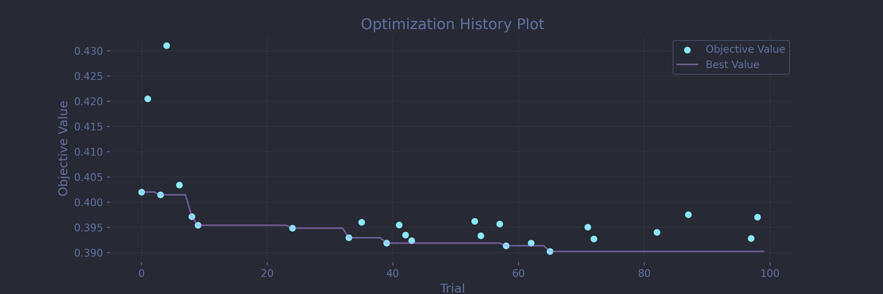
Keep in mind that despite setting all the usual random seeds, I wasn’t able to make PyTorch fully deterministic. Fortunately, thanks to the 5-fold cross validation, the run-to-run variance in accuracy is minor and the conclusions should remain meaningful. That being said, here are the result of the best trial Optuna recorded for this run:
Best trial:
Logloss: 0.39023858308792114
Params:
batch_size: 128
width: 496
depth: 4
lr: 0.01452463838833435
dropout_rate: 0.36297352311247777
epochs: 23
Optuna settled on quite a massive architecture for this small dataset: the depth of 4 and the width of 496 implies a total of over 1700 neurons in the hidden layers. This is compensated by ignoring the outputs of basically 1/3 of the neurons and overfitting is also kept in check through the small batch size and early stopping. The learning rate of roughly 0.015 looks reasonable. This overall is a pretty surprising configuration to me, but the validation score loss looks promising enough. And indeed, on a holdout test set, our network reaches above 0.8, almost putting it on par with the CatBoost model:
Accuracy: 0.7987349051178838
              precision    recall  f1-score   support

         0.0       0.75      0.88      0.81       856
         1.0       0.86      0.72      0.78       883

    accuracy                           0.80      1739
   macro avg       0.81      0.80      0.80      1739
weighted avg       0.81      0.80      0.80      1739
8. The Moment Of Truth: Final Evaluation
Both models have been tuned, and it’s finally time to train them on the full dataset. When I submitted the predictions to Kaggle, the CatBoost model scored 0.798, while the PyTorch neural network managed 0.801. Goal achieved! We successfully matched (and even slightly exceeded) our baseline with a neural network.
That said, it would be a mistake to conclude that neural networks inherently outperform tree-based models, especially on small tabular datasets like this one. With a bit more tuning, CatBoost could easily come back on top. In fact, by just changing the random seed, I once reached 0.80570, which placed me 210th out of 1,439 participants (top 15%) at the time of writing. And that’s our secondary goal accomplished: a respectable leaderboard position!

One interesting trick you can try is to combine the two models. Because their architectures are so different, they might make different kinds of mistakes. In this specific case, a naive average their prediction probabilities is a surprisingly effective way to combine their strengths:
ensemble_preds = (dnn_preds + gbt_preds) / 2
This simple ensemble consistently nudged the accuracy a bit higher than either model alone, reaching 0.80476 with SEED = 1
9. Peeking Inside the Black Box
I could have ended this article here. But by now, you probably know my weakness for interpretation and visualization. I like to see what’s happening and understand why it’s happening. And I firmly believe that if a picture is worth a thousand words, then an animation is worth the sum of all its frames.
That said, neural networks are notoriously hard to peek into. Still, there are a few ways to illuminate the black box just enough to let us see some of what’s going on, and that’s exactly what we’ll do in this final part.
Peering Into the Features
One of my first go-to plots for any machine learning model is a feature importance bar chart. It’s an excellent way to validate and guide your feature engineering work by showing what features the model focuses on most. Unfortunately, PyTorch doesn’t just hand us the feature importances data. Unlike tree-based models, where they can be derived directly from split statistics, neural networks are much more of a black box. Still, we can get a sense of which features matter most using a model-agnostic approach: permutation importance.
The idea is simple: measure your model’s performance using your favorite metric, then shuffle one feature column at a time (which breaks its relationship with the target) and re-evaluate. If performance drops sharply, that feature was important. If it barely moves, it wasn’t contributing much at all.
Scikit-learn makes this easy for any model that follows its API:
from sklearn.inspection import permutation_importance

result = permutation_importance(
    model, X_test, y_test,
    n_repeats=10, scoring='neg_log_loss'
)
importances = result.importances_mean
Making a pytorch model compatible with the Scikit-learn API is a bit tricky: you need to write a small wrapper class that implements the fit() and predict_proba(), and take care of a few other details as well. My code is available in the companion notebook if you’re curious. But for now, let’s just compare both models side by side:
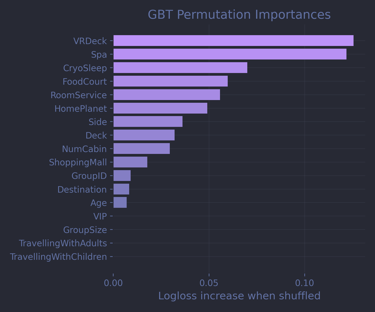
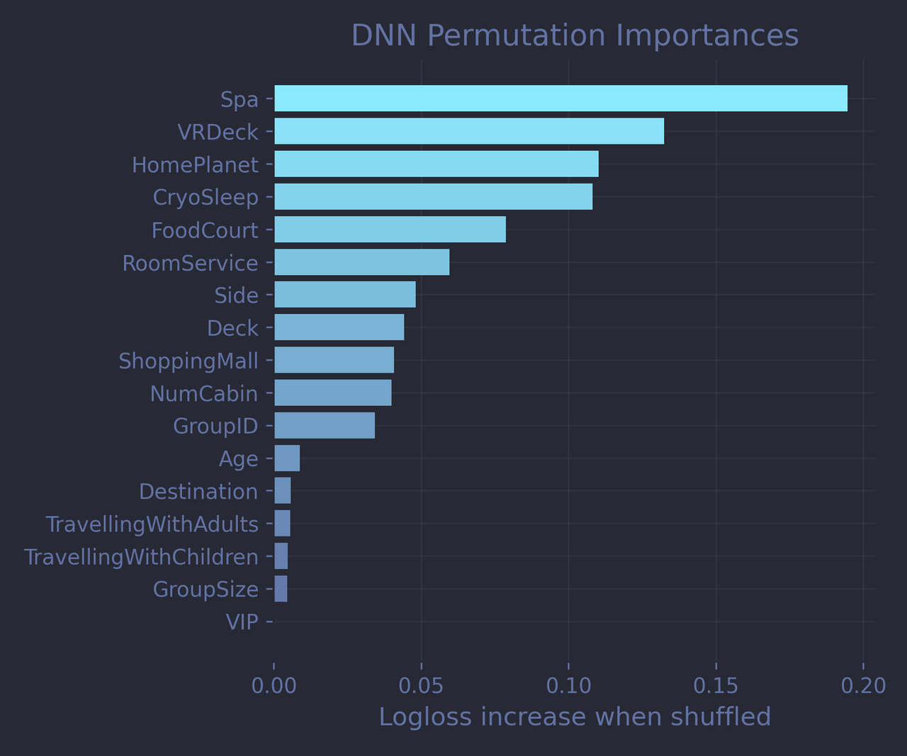
We should be cautious when comparing permutation importances across very different architectures. Still, the general story is consistent: both models agree that Spa and VRDeck are among the top predictive features, while, tragically, our lovingly crafted TravellingWithAdults and TravellingWithChildren features are deemed completely useless. It’s also tempting to credit the seemingly higher predictive power of HomePlanet according to the PyTorch model to our embedding work, though I’m not entirely sure I believe it.
I won’t go into all the details here, but just like with feature importances, it’s possible to compute SHAP values in a model-agnostic way using a similar permutation-based approach.
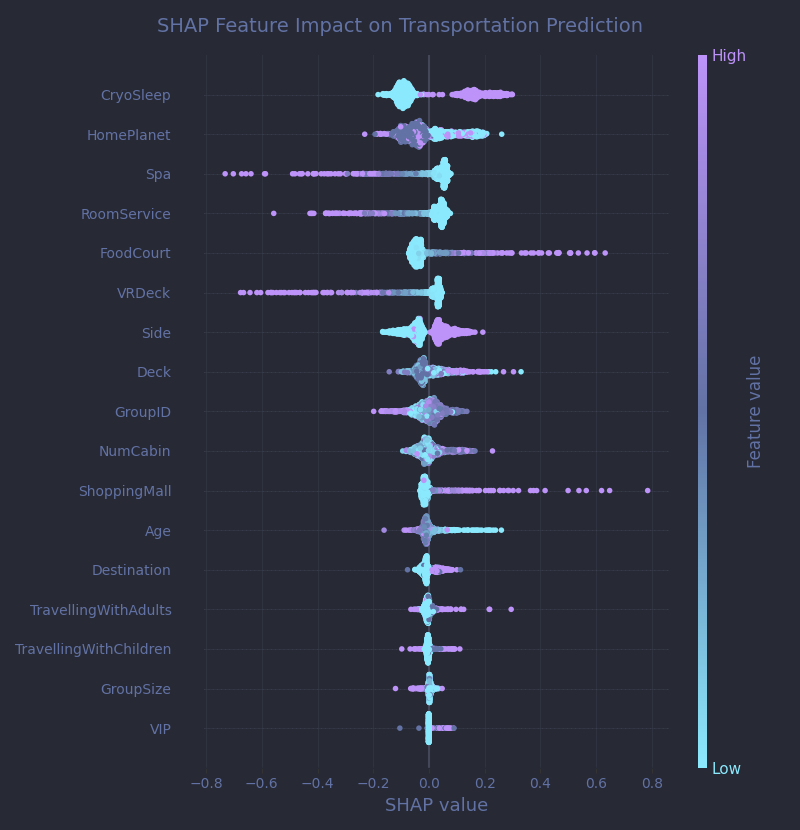
If you’re not familiar with this type of visualization, I covered the basics in my previous Titanic article. What stood out to me immediately here is how strongly the various spending features (VRDeck, FoodCourt, etc.) influence the predictions, but in opposite directions. Some Kaggle competitors suggest summing all those spending amounts into a single "total spent" feature. It sounds reasonable, so I tried it. My accuracy dropped by 5% instantly. And this plot makes it clear why: each spending category carries its own distinct signal, and merging them into one number completely flattens those differences.
Of course, so far, we have just been watching the final outcome in aggregate. What’s might even more fascinating is watching learning and inference happen in real time.
Neural Network in motion
Unfortunately, the best model selected by Optuna turned out to be quite wide, which makes any visualization difficult. So for the next animations, I limited each layer to 32 neurons. You’ll have to imagine that the final model is actually almost five times wider!
That being said, let’s start with learning.
To create this animation, I recorded the weights between layers at each batch during training. I then computed the highest weight across all layers and epochs, and varied each edge’s width, color, and opacity depending on how strong its weight was relative to that maximum. In practice, this means that stronger connections appear thicker, more colorful, and more opaque, allowing you to compare them across layers and epochs. The network is still fully connected, but I hid the edges corresponding to very low weights to reduce visual clutter.
As training progresses, the weights visibly strengthen, especially between the input layer and the first hidden layer. The colors grow more vivid and the lines thicker as the model becomes more confident about which connections matter most. The fact that later layers maintain moderate weight values is a good sign that our batch normalization setup is working, preventing weights from exploding or vanishing layer after layer. After a few epochs, the network settles into a stable structure. It’s also worth noting how some input neurons connect with stronger weights than others. This may be hinting at more predictive features, but it also may mean the those neurons carry on average a lower activation that the network had to compensate for with higher weights.
Let’s now take a look at what happens during inference—when the network has finished training and is in prediction mode. In this case, we’re predicting the transportation status of Nelly Carsoning, a 27-year-old passenger from Earth traveling to TRAPPIST-1e in cabin G/3/S, who hasn’t spent anything along the way. The network gives her a 0.52 probability of being transported.
In this animation, each neuron is color-coded by its activation—purple for positive, cyan for negative. The edges no longer represent weights but signals, which, as you remember, are the actual values flowing from one neuron to the next.
And now you see why neural networks are often called black boxes. It’s not that we can’t see what’s going on, it’s that what we see is so hard to interpret. From left to right, it looks like GroupID and CryoSleep play a major role in this particular case, with strong signals emitted from their corresponding neurons. After the second layer, all the signals fade progressively. Maybe it could be interpreted as the network lack of confidence in its prediction?
Let’s compare with a different passenger: Polar Extraly, a VIP traveler from Europa who spent quite a bit at the spa. The network gives him a 0.38 probability of transportation.
Here, the first-layer signals are easy to read: they are strong and numerous from the neuron corresponding to the Spa feature, confirming what we already know: spa spending is a powerful predictor. But after that, it’s chaotic. The only pattern that jumps out to me is that unlike Nelly’s case, the deeper layers seem to amplify the signals instead of damping them, giving weight to our theory of network self-confidence.
You could argue that these animations are a bit of an exercise in futility, given how little we can truly interpret from them, and you wouldn’t be entirely wrong. But I’m vain, and I like pretty colors and shapes moving around. I could watch them all day, and that alone justifies the absurd amount of time I spent writing that animation code (which you can check out on the GitHub repo!).
I also think they make a deeper point. They capture, visually, the challenge of interpreting neural networks. With decision trees, you can always extract individual decision trees and reason about each branch. With neural networks, the "rules" governing a single neuron's activation mean nothing in isolation and only make sense in the wider context of the whole network.
You might have heard somewhere in pop culture that AI is scary because we don't know how it works. We do know how it works, we wrote the damn code and we can output parameters and activations anytime we want! What is difficult to say is why it works at the individual neuron level.
Conclusion
I know this one was a long read, and I am truly sorry about that, but there was a lot to cover. I am always tempted to stick to the basics, but those can be found everywhere on the internet. I feel the real value here lies in going a bit deeper while keeping things understandable, even for the curious non-professional. I hope I managed to do just that. I find neural networks fascinating, and I believe that even if you never plan to train or deploy your own, having at least a surface-level understanding of how they work should be part of everyone's general knowledge in our modern world.
As always, you are more than welcome to check out the full Jupyter notebook, as well as a streamlined and heavily commented Python script on the GitHub repo.
And finally, let me thank you for sticking with me until the end. Writing this article has been a lot of work, but if you enjoyed reading it even half as much as I enjoyed making the animations, it's a win in my book.